
Apple silicon chips provide several options for high-performance vector and matrix computation, including the NEON unit in each CPU core, which I examined in the last article in this series, the GPU and neural engine (ANE), and Apple’s own matrix coprocessor, the AMX. For most of these, Apple provides libraries that deliver the best performance appropriate to the hardware platform they’re run on. Apple doesn’t as a rule document which of those any given function will use.
AMX is intentionally undocumented, and its existence in Apple silicon chips remains shrouded in mystery. Research has documented the instruction set for M1 and M2 family chips, but precious little is known about the AMX coprocessor(s) in the M3 family. I’m very grateful to Maynard Handley, who suggested that I incorporate two test routines for use on the M3 Pro to try to elicit information about its AMX performance.
This article relies on explanations of the methods used in previous articles in this series:
If you’re not already familiar with the first of those, I recommend that you read it before this article, or you may well be mystified.
Tests
Results reported here come from two new tests that I have incorporated into my GUI wrapper app, both drawn from Apple’s Accelerate library, one from vDSP and the other a Sparse Solver. The code, given in full in the Appendix at the end, has been shamelessly stolen from Apple’s documentation.
The vDSP test performs a forward fast Fourier transform and an inverse transform on eight real elements, using two calls to vDSP_DFT_Execute(). The original example is given here. The Sparse Solver test uses a sparse Cholesky factorization, then uses that to solve its equation with SparseSolve(). Its original example is given here.
vDSP FFT
The relationship between the rate of executing vDSP FFT test loops and the number of threads is quite unlike any other that I’ve seen during testing. For 1-4 threads, this follows a linear relationship as seen generally, but the throughput rate then falls when going from four to five threads (cores). From five threads upwards, the relationship is again linear, but with a lesser gradient than with fewer threads.

This is shown clearly in the chart above, where results for the P cores in an M1 Max are shown in blue, and those from the P cores in an M3 Pro are in red. For both line segments, the gradient attained by the M3 is significantly steeper than that for the M1: the M3 Pro throughput was 135% that of the M1 Max, and the ratio of gradients is almost the same. However, at higher thread numbers, the M3 Pro achieved over 170% of the throughput of the M1 Max.
The reason for this fall in throughput when going from 4 to 5 threads isn’t clear, bearing in mind that the M1 has four-core clusters but the M3’s clusters contain six cores. Looking in detail at powermetrics measurements for the M3 Pro, there was a small reduction in P core frequency, from 3624 with 1-4 threads to 3576 with 5 threads, but that’s insufficient to account for the difference seen.
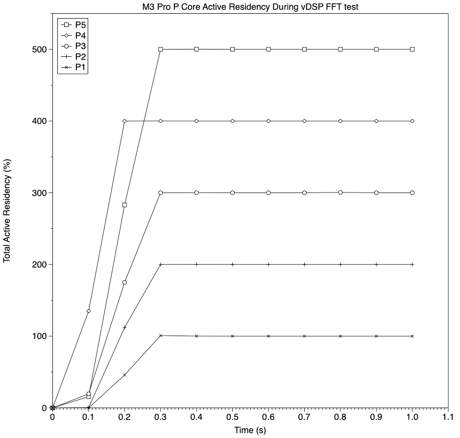
This chart of total active residency for the six-core P cluster demonstrates that each thread added a single core’s worth of 100%, and with five test threads total active residency remained at 500%, well within the maximum total of 600% for the cluster.
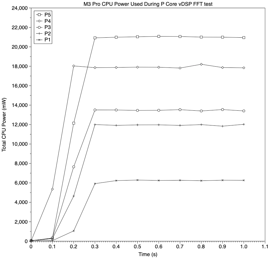
There is something going on with these tests, though, as suggested by this chart of total CPU power used for 1-5 threads. Instead of being evenly spaced, they’re quite irregular and almost grouped in pairs. Note that powermetrics gives separate estimates for CPU and neural engine power, both of which remained close to zero throughout, but doesn’t make it clear whether AMX power use is included in its total CPU figures.
Whatever the reasons, the behaviour of the vDSP FFT test is very different from other tests that I have used, apart from the next.
Sparse solver
If the throughput of the vDSP FFT test looked incoherent, that from the Sparse Solver test appears almost random.
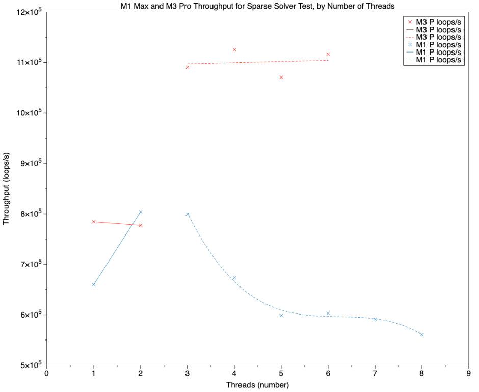
Once again, in this chart blue points and lines are those of the M1 Max, and red are from the M3 Pro. Here there’s a marked discontinuity between two and three threads. Above three threads, the M1 appears to decline steadily, while the M3 is far higher and relatively steady.
On the M3 Pro, core frequencies were lower at 3516 MHz with one and two threads, and rose to 3580-3590 MHz with three and four threads, another difference too small to account for the changes seen in throughput.
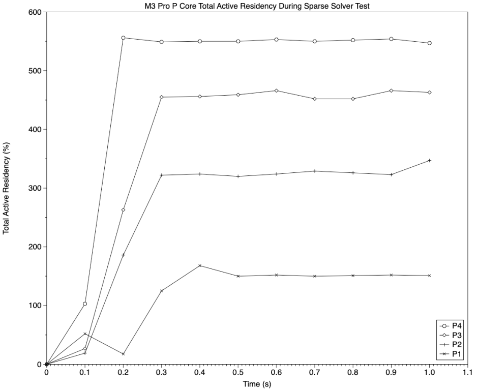
Active residency was different from the vDSP FFT test, as it was significantly greater than that of the test threads alone. With a single test thread of 100%, total active residency on the cluster of P cores was about 150%, and with four threads totalling 400%, overall active residency totalled about 550% for the cluster. This would account for falling throughput with five threads or more, as they would exceed the 600% available from the P cores, but it doesn’t explain behaviour with four threads or less.

Total CPU power was also irregular, suggesting something else is going on, as with the vDSP FFT test.
Different tests
Because the AMX coprocessor can only be used through Apple’s libraries, and it’s unclear which of their functions do perform their computation on the AMX, it’s not possible to conclude these results tell us anything about the AMX in either of these chips.
Code run in these tests is considerably more complex than the tight loops of assembly language I have used previously. Both test functions involve substantial overhead in terms of setting up variables both before the test loop and within it. Even moving as much as possible outside the loop, memory access from code inside the loop is inevitable.
In the Sparse Solver test, test code incurred substantial processing outside the test thread, sufficient to require an additional 50-150% active residency, and limit the six-core cluster of the M3 Pro to running a total of only four threads. While it’s possible that additional processing is required to support code running on the AMX, more information is required.
These two additional tests demonstrate how difficult it is to gain insights into core or coprocessor performance when running more complex code, and how useful tight code loops are by comparison.
Performance
If there’s one observation that shines through these clouds, it’s how performant the M3 Pro is when executing demanding tasks such as fast Fourier transforms and Cholesky decomposition. Relative to those of the M1 Max, throughputs of the M3 Pro attained 135% (FFT, low thread count), over 170% (FFT, high thread count), and 140% (Sparse Solver). Those can be attributed to the Accelerate library, the AMX coprocessor, improved core management and other factors, but teasing those apart requires much more work.
Conclusions
- Interpreting the results of more complex tests is far harder because there are too many unknown and uncontrolled variables.
- Throughput of vDSP FFT and Sparse Solver tasks shows complex relationships with the number of test threads.
- Both tests showed discontinuities in the relationship between throughput and thread count, although at different points: for the FFT, it occurred between 4-5 threads, whereas the Sparse Solver discontinuity was between 2-3 threads, in a six-core cluster.
- Relative to the M1 Max, the M3 Pro generally attained substantially higher throughput, ranging from 135% to over 170%.
- Although it’s impossible to identify the factors responsible, the AMX coprocessor may well have contributed to those differences.
Appendix: Source code
func runvDSPFFT(theReps: Int) -> Float {
let realValuesCount = 8
var theCount: Float = 0.0
var complexReals: [Float] = [0, 2, 4, 6]
var complexImaginaries: [Float] = [1, 3, 5, 7]
for _ in 1…theReps {
if let dft = vDSP_DFT_zrop_CreateSetup(nil, vDSP_Length(realValuesCount), .FORWARD) {
vDSP_DFT_Execute(dft, complexReals, complexImaginaries, &complexReals, &complexImaginaries)
vDSP_DFT_DestroySetup(dft)
}
vDSP.multiply(1 / 2, complexReals, result: &complexReals)
vDSP.multiply(1 / 2, complexImaginaries, result: &complexImaginaries)
if let dft = vDSP_DFT_zrop_CreateSetup(nil, vDSP_Length(realValuesCount), .INVERSE) {
vDSP_DFT_Execute(dft, complexReals, complexImaginaries, &complexReals, &complexImaginaries)
vDSP_DFT_DestroySetup(dft)
}
vDSP.multiply(1 / Float(realValuesCount), complexReals, result: &complexReals)
vDSP.multiply(1 / Float(realValuesCount), complexImaginaries, result: &complexImaginaries)
theCount += 1
}
return theCount
}
func runSparseSolver(theReps: Int) -> Float {
var theCount: Float = 0.0
var columnStarts = [0, 3, 6, 7, 8]
var rowIndices: [Int32] = [0, 1, 3, 1, 2, 3, 2, 3]
var attributes = SparseAttributes_t()
attributes.triangle = SparseLowerTriangle
attributes.kind = SparseSymmetric
let structure = SparseMatrixStructure(rowCount: 4, columnCount: 4, columnStarts: &columnStarts,
rowIndices: &rowIndices, attributes: attributes, blockSize: 1)
var values = [10.0, 1.0, 2.5, 12.0, -0.3, 1.1, 9.5, 6.0]
var bValues = [ 2.20, 2.85, 2.79, 2.87 ]
var xValues = [ 0.00, 0.00, 0.00, 0.00 ]
for _ in 1…theReps {
let llt: SparseOpaqueFactorization_Double = values.withUnsafeMutableBufferPointer { valuesPtr in
let A = SparseMatrix_Double(structure: structure, data: valuesPtr.baseAddress!)
return SparseFactor(SparseFactorizationCholesky, A)
}
defer { SparseCleanup(llt) }
bValues.withUnsafeMutableBufferPointer { bPtr in
xValues.withUnsafeMutableBufferPointer { xPtr in
let b = DenseVector_Double(count: 4, data: bPtr.baseAddress!)
let x = DenseVector_Double(count: 4, data: xPtr.baseAddress!)
SparseSolve(llt, b, x)
} }
theCount += 1
}
return theCount
}
