So, having compressed text very efficiently, and managed to do quite well with images, I turn now to compressing audio.

Conversion to digital

Real-world audio input is, of course, analogue and not digital. So the first step to consider is how this will be converted into digital form.

Analogue audio can be represented as a complex waveform. In some cases, such as a single sustained note on a violin, this is close to being a pure ‘sine’ wave which could be expressed directly in mathematical terms. But in the vast majority of cases the only practical way of expressing it digitally is by sampling the waveform at discrete time points.

Although some people claim to be able to sense sound beyond the range heard by normal humans, the standard range of audio frequencies which we need to be able to represent faithfully in digital form is 20 to 20,000 Hz, with our most sensitive hearing range around 2,000 to 5,000 Hz.

Just after the Second World War, Harry Nyquist and Claude Shannon discovered and proved that in order to reconstruct a waveform accurately (such as when you convert it from digital back to analogue form, for example for audio output) you must sample the analogue waveform at a frequency of at least twice the maximum frequency which you need for reconstruction. (This is an important early discovery in information theory: the Nyquist-Shannon Sampling Theorem.) So for normal human hearing, the lowest sampling rate which we can use is 2 x 20,000 = 40,000 Hz.

In practice a little headroom is allowed, and basic digital audio should be sampled at 44,100 Hz. Professional audio conversion often uses higher frequencies, of 48,000 or even twice that, 96,000 Hz, in order to maintain the highest quality throughout, as it may be necessary to convert that audio several times before its processing is complete.

Non-lossy

Analogue to digital conversion of audio signals therefore results in a high-frequency stream of numbers representing the original analogue sound waves: data which is quite unlike those of text or images, so requiring a very different approach if we are to achieve worthwhile compression. The sample audio file used in this article, which uses 24 bits (3 bytes) per sample at a sample rate of 44,100 Hz over two channels (stereo), lasts 1 minute and 40 seconds, and in uncompressed (WAV) format occupies 26.5 MB.

Lossless compression methods analyse the audio signal. Where they find blocks of identical sample values, such as during silent passages, they use run-length encoding for those. FLAC (free lossless audio CODEC) then uses linear prediction techniques through the stream of samples, producing a stream of predictor values, and another stream consisting of the difference between predicted and actual values, known as the residual. The latter stream is then encoded further (using Rice-Golomb encoding), and the two streams form the compressed output.

This may not appear particularly efficient, but in practice most audio files are shrunk to about half their original size: in this case, the compressed FLAC file is 18.5 MB or 70% of the original size. Here is that FLAC file:

Compo1

Lossy

For audio to be widely playable on small portable devices, better compression is required, or the storage requirements for even modest music libraries would be excessive and costly.

Research during the twentieth century has shown that we do not perceive all sound within our normal hearing range. For example, some sounds mask out others. As a result, psychoacoustic models have been built, which form the basis of most forms of lossy audio compression: they literally discard the audio information which the models predict we will not hear.

MP3 (MPEG-2 Audio Layer III) compression was developed in the early 1990s to apply psychoacoustic models to efficient audio compression, and has flourished since. Unlike most standards, it does not lay down exactly how this is to be achieved, but provides example models which are implemented in different ways by various CODECs. Thus some perform better than others under different conditions.

Encoding involves division of the audio stream into blocks, typically 576 samples long. Each is analysed in terms of frequency, and various filters applied. There are several controls over the amount and type of filtering used, but the main user choice is whether to set a constant or variable bit-rate, and what that rate should be. Together these set the amount of compression.

Variable bit-rate allows the CODEC to compress silences and ‘simple’ passages very highly, and to retain detail in more ‘complex’ passages, and therefore normally results in the best quality for the given compressed file size. Constant bit-rate was more popular when MP3 players were less capable, and could only manage to play back at a steady rate.

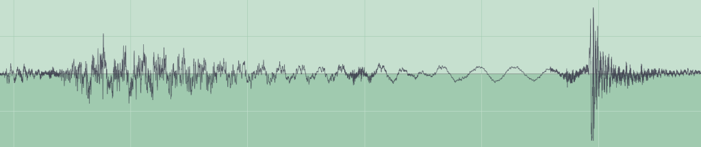
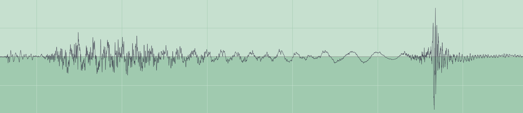
Today the standard bit-rate for MP3 compression of music is 128 kbits per second, and as the rate falls below that more and more listeners will notice deterioration in sound quality. You can see this by comparing the original audio waveform (encoded without loss using FLAC) with that in a 16 kbits per second MP3 compressed version.

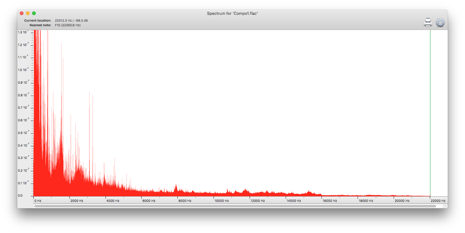
The effects are even more obvious when looking at an average frequency spectrum, for the same audio using FLAC lossless, a constant bit-rate of 64 kbits per second, and one of 16 kbits per second.

Audio samples, which contain psychoacoustic examples and a range of different types of music, are provided here too. The FLAC lossless sample (above) is packaged in Zip form (although that did not produce any further compression).

A variable bit-rate MP3 version is almost indistinguishable, as is a constant bit-rate of 128 kbits per second. When the bit-rate is reduced to 64, there is noticeable alteration of some of the test sounds, which is worse at 32, and dreadful at 16 kbits per second.

Variable bit-rate:

Constant bit-rate, 128 kbits/s, quality 2:

Constant bit-rate, 64 kbits/s, quality 2:

Constant bit-rate, 32 kbits/s, quality 2:

Constant bit-rate, 16 kbits/s, quality 2:

Using a variable bit-rate, the compressed file size is 2 MB (8% of raw size), falling to 1.6 MB at a constant bit-rate of 128, 802 KB at 64, 401 KB at 32, and 201 KB (0.7% of raw) at 16 kbits per second.

As with JPEG compression of images, to ensure the highest compression without detectable reduction in quality, you need to try different compression options, including constant versus variable bit-rate, target bit-rate, and the ‘quality’ settings. However with audio it is much harder to make quick comparisons, and most users simply choose settings which seem to perform reasonably well, and stick with those.

This can be dangerous, as the final sample of gamelan music shows. Early during the development of lossy audio compression, it was realised that gamelan music was usually a good test case, because of its rich sonorous and percussive sounds, which are at the limits of most psychoacoustic models. Normally, if your MP3 compression settings ensure acceptable quality in gamelan tracks, they will work well for most other types of music too.

Finally, for human speech to remain intelligible, you can use much lower bit-rates and thus achieve much greater compression, as well as applying bandwidth filtering.

Gamelan music by Gamelan Mitra Kusuma, excerpted from Archive.org.